Short Run Price Adjustment
Bengt Assarsson
2004-06-21
As noted in the description of the long run equilibrium general price level it is likely that the price level in the short run will deviate due to short run price rigidity. This must be handled somehow in any model that wants to describe actual behaviour reasonably well. Most equations in BASMOD are estimated in error correction form. This often means that the long run equilibrium is contained in the error correction term (or mechanism) and that the short run dynamics is estimated freely and “without theory”. This is of course unsatisfactory in some sense but may be reasonable in a situation in which there is much uncertainty both about the theory and about how to implement it empirically (which seems to be the case here).
The solution chosen here is based on the theory proposed by Ball and Mankiw (1994,1995) in which they develop a model in which inflation is explained by higher moments of relative- price changes. Their theory is based on the assumption of short run price rigidities in at least some sectors of the economy. The relationship between these higher moments and the rate of inflation can however be explained by other factors than price rigidity which has been explained by Balke and Wynne (1998) – in the case of productivity shocks – Bryan and Chechetti (1996) – in the case of a statistical bias – and by Assarsson (2003) in the case of cyclical shocks and the durability of goods. In practice the relationship between inflation and the higher moments of relative-price changes can be caused by many factors which may be present simultaneously. However, we prefer here to interpret the results in terms of price rigidities since these have been established elsewhere – see Assarsson (1989), Blinder (1993) and Apel, Friberg and Hallsten (2001).
The basic idea in Ball and Mankiw is that it takes large shocks to change prices quickly. Firms with costs for changing prices (which is virtually every one) do not find it worthwhile to change price unless the benefit (coming closer to the optimal price) is at least as big as the cost of changing the price. Hence, when the shock is small some firms find it optimal to keep the price unchanged while if the shock is large the benefit of changing the price outweighs the cost.
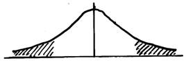
Diagram 1. A symmetric distribution of relative-price changes.
Diagram 1 depicts a symmetric distribution of relative-price changes. By definition, the mean is equal to zero, since the relative-price change is defined as and is the mean of the prices or price indices and is the budget share for the ith good. For a symmetric distribution there would be as many price increases as there are price decreases subject to the supply shocks that occur. Only shocks that are big enough cause prices to actually change and those shocks are shown in the shaded area in the diagram. The unshaded shows a range of inaction in which shocks are so small that they don’t warrant any price changes. In the case of a symmetric distribution the shaded areas to the left and right of the center of the distribution are equally large. This implies that the skewness of the distribution is zero and then inflation is unaffected.
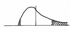
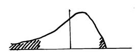
Diagram 2. Positively skewed (upper part) and negatively skewed (lower part) distribution of relative-price changes.
Now consider the case of skewed distributions as in diagram 2. As with the symmetric distribution the mean of relative-price changes is still zero but the skewness no longer is. In the case of a positively skewed distribution (as in the upper part of the diagram) there are a few very large increases (negative supply shocks) that are matched by many small decreases (positive supply shocks). In theory the supply shocks are not realized but Ball and Mankiw show that the distributions of unrealized supply shocks can be translated to realized relative-price changes. The few large negative shocks then cause price increases while the many small positive shocks do not. The effect is that positive skewness of relative-price changes adds to the rate of inflation while negative skewness decreases inflation. Therefore, the skewness of relative-price changes could account for the effects of short run price rigidity and help improve Phillips curves or otherwise standard price equations.
A typical Phillips curve would be based on the idea that the price level is a markup on marginal cost of the type as explained in the section about the long run equilibrium general price level. If we denote the long run price level determined by that model as a possible error correction model is:
(1)
with almost obvious notation[1]. Such a model can be extended and improved by including the skewness of relative-price changes. Define the skewness as
(2)
where
(3)
is the variance of relative-price changes.
Ball and Mankiw also extend their model somewhat and show that there is a role also for the variance. They show that the effect of the skewness of relative-price changes on the rate of inflation depends on the variance. A large variance magnifies the effect from skewness.
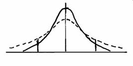
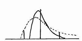
Diagram 3. The interaction of variance and skewness.
This can be seen in diagram 3. In the upper part an increase in the variance of shocks affects the tails symmetrically and consequently has no effect on inflation. In the lower part, where the distribution is asymmetric, an increase in the variance has a larger effect on the right-hand than on the left-hand tail and hence strengthens the effect of skewness on the rate of inflation.
For most industrialized countries inflation has been positive the past decades (trend inflation). With trend inflation it can be shown that skewness tends to be positive also in the long run and that the variance of relative-price changes in itself is positively related to the rate of inflation. With trend inflation there will be an asymmetric range of inaction which shifts to the left. The reason is that trend inflation implies that desired price decreases to some extent can be carried out with constant prices. The implication is that an increase in the variance of relative-price changes adds to inflation even if the distribution is symmetric.
The price equation then can be altered:
(4)
such that we include the skewness and variance of relative-price changes as well as the product of these higher moments in an otherwise typical equation.
The results from estimating price equations with and without the higher moments can be studied in The Econometrics of Higher Moments and the Phillips Curve.