Basic user manual

 

1 How to Get Started

 

Download the model from

 

S:\APP\APP Modellenheten\BASMOD\BASE\0402\basmod0402.wf1

 

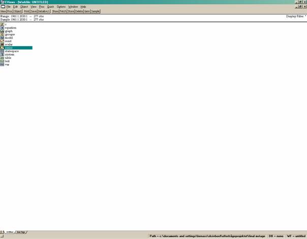
to your appropriate directory and start Eviews. Click on Model in the workfile and the following screen appears

 

 

To the left we have the Workfile window and to the right the Model window. There are different views in the Model window and it is the Equations view that appears above. From the Equations view you can view the equations, add shocks or exogenise variables. In the Variables view

 

 

you can view the variables, create diagrams and tables. Note the Filter/Sort and Dependencies buttons in the upper left of the window. There you can sort the variables according to type (like exogenous, endogenous) or show which variables X depends on or variables that depend on X.

 

We now click on the Solve button to get

 

 

Click on Solver to get

 

 

where you click on Previous period’s solution and on Constant growth rate. Then you go back to the Basic Options sheet and click OK. The model solves Scenario 2 and you’re on to it running BASMOD.

 

You can view the results by viewing the variables for Scenario 2, e.g. @pcy(sey_2) which is the annual growth rate for GDP in Scenario 2. You can also view the results in the Variables view, where you can create graphs and tables and transform the variables, e.g. from levels to annual growth rates.

 

2 The setup in Eviews

 

It is useful to be aware of the basic concepts in Eviews. To begin with you start with a so called Workfile which is a file in Windows operating system with extension .wf1. Eviews also recognises program files with extension .prg and text files with extensions .txt. However, operations take place within the workfile where you refer to various Objects. Eviews deals primarily with time series and consequently one object is Series. The variables in BASMOD are Series. The different Eviews objects that are used in BASMOD and stored in the Workfile can be listed:

 

·        Series

·        Scalar

·        Coef

·        Group

·        Graph

·        Text

·        Equation

·        System

·        VAR

·        Sspace

·        Model

 

You open an object by double-clicking on the object in the Workfile. The object then opens in a new window. The exception is the Scalar object that only shows its value in the lower left corner of the Workfile window. It has a yellow icon with a #. The Coef object is a coefficient vector and has a yellow icon with a . A group is a number of objects, presumably a number of Series and is shown by a yellow icon with a G. There are also Graph, Text and Table objects.

 

 

 

Then there are the objects

 

·        Equation

·        System

·        VAR

·        Sspace

·        Model

 

The Equation object shows a single estimated equation. The equation can use different estimators and can be linear or nonlinear. The System object refers to a system of estimated equations which also can use different estimators and be linear or nonlinear. The VAR object is a special case of System that uses certain predefined procedures to produce impulse responses, variance decompositions, etc. The SS or Sspace object is a state space model in which you can define models with time varying parameters.

 

The Model object is a system of equations which can be solved for the endogenous variables given the values of the exogenous variables. The model can be static or dynamic and deterministic or stochastic. The model is written down in a text file which is contained in the Model object, i.e. you can start a new model object and write it down it the text module of the object and then save it. Identities such as the GDP identity

 

 

is simply written down in the text module of the Model object, while estimated equations are linked to the model. The aggregate consumption function is named ekc and the text module may then look like

 

‘ This is the consumption function and the GDP identity

:ekc

 

in the text module. A comment line is preceded by the ‘. The linking is done by the colon :

 

It is easy to change the specification in the model by reestimating or replacing equations. If you have an alternative consumption function you just replace ekc with the name of the alternative equation.

 

Let’s have a closer look into the Model object.

 

 

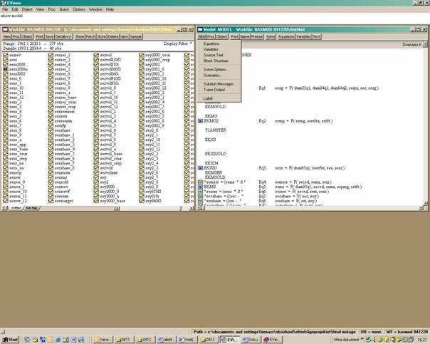
Above we see two open windows, the Workfile to the left and the Model to the right (the model object is named Model). There are 10 buttons by which you can change between different views.

 

The equations button lets you view and get summary information about the equations of the model, which is shown below.

 

 

 

 

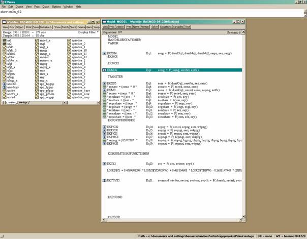
Here the dependencies are shown in the same form as above, e.g. sexshare = F(sex,sey) shows that the contribution of exports to GDP growth – sexshare – depends on exports – sex – and GDP – sey. Estimated equations are shown with a blue = icon and equations that are definitions or identities are shown with a green txt icon.

 

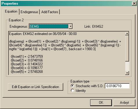
If you click on one of the equations, e.g. the EKMG2 for imports of goods, you find information about the equation under the Equation tag; the estimated parameters and the standard error of the regression reported in the lower right corner.

 

The other two tags – Endogenous and Add Factors – are useful when running simulations and forecasts – see section 3.4 below.

 

An alternative way to inspect the equation is to click on EKMG2 in the workfile window. The equation view then appears and a lot of detailed information about the specification is available. Of course, you can then perform various econometric tests with the equation, inspect residuals, etc. You can also re-estimate the equation and link it to the model.

 

 

 

Return to the main menu and click on the Text button. The model as “it is actually written” appears in the window. Here you can revise the model by changing the text and linking various equations, systems of equations, VARs or state space models. For instance, in BASMOD some foreign variables are exogenous but if you prefer you can estimate a VAR named Foreign with the foreign variables and link it to the model through

 

:Foreign

 

and then run the model with the foreign variables as endogenous. Similarly, if you believe that the effect of wealth on private consumption changes over time you can estimate the consumption function in the state space form with the name Change and link it to the model by

 

:Change

 

 

To view the objects in the model you can simply click on them in the workfile window. In the workfile window you can also store some objects that are presently not part of the model, perhaps in the event of using them later. An alternative is to view the model objects through the Variables button in the Model view:

 

 

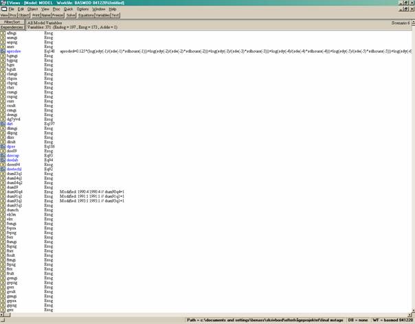
There are three types of variables in the model, endogenous, exogenous and add factors (which are also exogenous). You can sort the variables according to that or in alphabetical order by series name. Click on Filter/Sort:

 

 

 

 

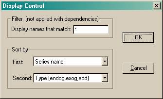
and you can choose how to sort the variables according to name, type or equation number. Another useful tool is to find out about the dependencies between the variables. Find the SEC variable which is private consumption expenditure, highlight it and then Click on the Dependencies button to get

 

 

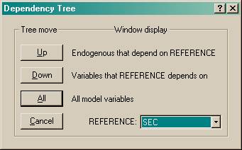
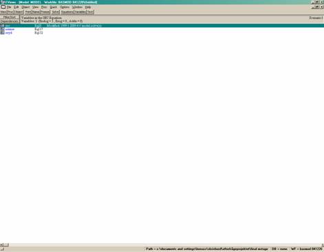
Click on the Down button and you can find out which variables that private consumption expenditure depends on, i.e. on total real net wealth and real private disposable income:

 

 

 

If we instead Click on the Up button we can find out which variables SEC affects:

 

 

 

Within the Model view we can also view the variables in graphs and tables. Double-Click on two variables, SEBI and SEC. to open them (in a Group window). Choose the View button and you can show graphs and create tables. Choose Dated Data Table to create a table and click on the Tab Options button to get the Table Options menu.

 

 

Here you can transform the variables from levels to quarterly or annualised percentage changes or to one year percentage changes which is very useful.

 

Solving the model

 

To solve the model you click on the Solve button in the main menu of the Model view to get

 

 

Among the Basic Options are to choose between determinstic or stochastic and dynamic or static solutions. Since the model is forward-looking it cannot be solved in the stochastic mode in Eviews. Normally, you would also choose the dynamic option, though the static mode can be used to evaluate the model’s fit within the sample. A solution of the model always creates a numbered scenario and the solved variables given the extension _6 in the above example – e.g. SEY_6 for GDP in this example. The Solver tag gives further options:

 

 

 

Since the model is solved forward some solution must be reached for the forward-looking variables beyond the forecast horizon. For instance, if the model is solved until 2018:4 and wages depend on the expected prices four quarter ahead there must be a solution for prices up to 2019:4. This can be solved by assuming a constant growth rate from 2018:4 and onward or by giving exogenous values for the terminal year (User supplied in Actuals). I normally run the model with the former option, as in the example above.

 

Click on OK, the model runs and you probably get a message like

 

 

 

You can then study the outcome for Scenario 6, possibly comparing with some other scenarios.

 

3 Data

 

Data are quarterly and mainly collected from the Nigem database, which is updated four times a year. The exogenous variables are mainly foreign variables. BASMOD uses the forecasts of Nigem for the foreign variables. Appendix A2.3 describes how to update the data base in BASMOD from the data base in Nigem. In addition, some variables are updated “manually” as they appear more frequently or are so important that they are updated prior to the update of Nigem. The manually updated variables are

 

·        National accounts balance of resources

·        Disaggregated private consumption data

·        Some labour market data from APP

·        Financial data like interest rates and equity prices

·        Consumer prices

·        House prices

·        Miscellaneous data such as housing starts, confidence indicators, etc.

 

Some of the data are annual, such as tax revenues, and are transformed to quarterly data. Some data are seasonally adjusted by Niesr in case collected from the Nigem data base and often the adjustment then has been done by the statistic authority – Statistics Sweden mostly – but occasionally also by Niesr. Some variables – such as the components of investments – have been seasonally adjusted in Eviews – with the X12 historical method (see Eviews for details). The list of variables can be found in Appendix 2.

 

4 How to make forecasts and simulations

 

Conditional forecasts in APP

 

Making a forecast with BASMOD is creating a scenario by solving the model, as shown above. Often simulations are conditional – e.g. on a constant policy rate of interest. Let us look at a typical forecast as done in the APP at the Riksbank. We are about to make a forecast for the Policy Report in 2004:4. We have data up to 2004:2 for the National Accounts and for interest rates and some financial variables until 2004:3. We run three separate forecasts depending on assumptions on the repo interest rate: constant until 2009, following the implicit market rate of interest and being endogenous in the model.

 

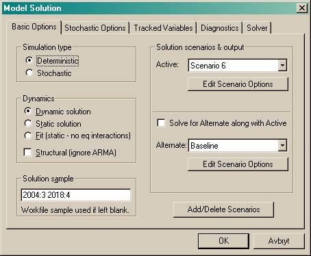
We start the forecast in 2004:3, i.e. assume that in general data until 2004:2 are available. However for some variables data are available also for 2004:3. We then exogenise these variables for 2004:3. For SEHW, housing wealth, this is done by clicking the Equations button in the Model view and then open the SEHW equation EKHW, with the Endogenous tag:

 

 

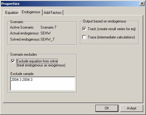
Exogenise SEHW for 2004:3 and run the forecast from the same period:

 

 

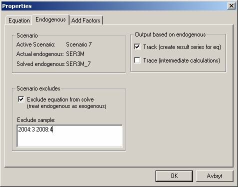
Do the same for other variables with the most recent data, perhaps even for 2004:4 for some variables.

 

To run the forecasts conditional on monetary policy we use different interest rate rules. The endogenous rule is the most simple. We use the following rule written in to the Text view of the Model object:

 

SER3M  = .67  * SER3M(-1)  + 1.5  + 1.2  * ((1  / 55)  * (@PCY(SEKPI80(+1))  - 2)  + (2  / 55)  * (@PCY(SEKPI80(+2))  - 2)  + (3  / 55)  * (@PCY(SEKPI80(+3))  - 2)  + (4  / 55)  * (@PCY(SEKPI80(+4))  - 2)  + (5  / 55)  * (@PCY(SEKPI80(+5))  - 2)  + (6  / 55)  * (@PCY(SEKPI80(+6))  - 2)  + (7  / 55)  * (@PCY(SEKPI80(+7))  - 2)  + (8  / 55)  * (@PCY(SEKPI80(+8))  - 2)  + (9  / 55)  * (@PCY(SEKPI80(+9))  - 2)  + (10  / 55)  * (@PCY(SEKPI80(+10))  - 2))

 

which says that the short run 3 months interest rate is set with respect to deviations of the expected from the target rate of 2 percent inflation up to 10 quarters ahead. Next, we run the model with the constant interest rate up to 2008. We then set SER3M to the present level 2.01 in the data and exogenise the above equation:

 

 

 

Using the implicit forward rates we simply create the series SER3MIT and solve the model accordingly. This is simply accomplished with these lines

 

 

’SER3M  = .67  * SER3M(-1)  + 1.5  + 1.2  * ((1  / 55)  * (@PCY(SEKPI80(+1))  - 2)  + (2  / 55)  * (@PCY(SEKPI80(+2))  - 2)  + (3  / 55)  * (@PCY(SEKPI80(+3))  - 2)  + (4  / 55)  * (@PCY(SEKPI80(+4))  - 2)  + (5  / 55)  * (@PCY(SEKPI80(+5))  - 2)  + (6  / 55)  * (@PCY(SEKPI80(+6))  - 2)  + (7  / 55)  * (@PCY(SEKPI80(+7))  - 2)  + (8  / 55)  * (@PCY(SEKPI80(+8))  - 2)  + (9  / 55)  * (@PCY(SEKPI80(+9))  - 2)  + (10  / 55)  * (@PCY(SEKPI80(+10))  - 2))

 

SER3M=SER3MIT

 

where the ’ sign rules out the previous interest rate rule.

 

 

Simulations

 

Simulations show how one or more shocks affect the outcome of all the variables in the model. Shocks can be imposed in many different ways. For the historical data period(s), shocks appear as residuals from the econometric estimations. When you run a forecast or simulation it can be stochastic and normally errors will be drawn from distriubutions inferred from the errors of the estimations with historical data. Errors for the forecast period can also be so called add factors which may emanate from the desire to affect the forecasts by judgements or to adjust the forecasts from anomalies. Forecasts in BASMOD are generally run without add factors and the forecasts are deterministic in the sense that all residuals in the forecast period are assumed to be equal to their historical means, i.e. zero. However, the user may very well use add factors but should then note that it affects how shocks should be inferred in the model.

 

Divide shocks into four different categories:

 

 

	Endogenous	Exogenous
Permanent	I	III
Transitory	II	IV

 

For any endogenous variable y suppose

 

 

where a and b are parameters,  is a variable that explains y and  is a disturbance term, an add factor in the Eviews language. A transformed dynamic version could typically be

 

 

Hence, usually . A shock is introduced in the forecast period by just adding an add factor different from zero. 

 

Click on the Add Factors tag and the following window appears in which you click on the Equation intercept (residual shift) followed by a click on Initialize Acitve Add Factor:

 

 

 

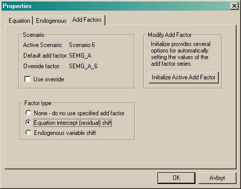
You are then prompted to initialize the add factor – in this example for the imports of goods – in the following window:

 

By clicking on So the this equation has No Residuals at ACTUALS you create the add factor SEMG_A which is an exogenous variable in the model and is equal to zero for the forecast period 2004:3 – 2018:4. Now you can edit this variable. Since the imports of goods equation is estimated in logarithmic form you can add a temporary one percent shock in the imports of goods in 2004:3 by opening the SEMG_A variable and add 0.01 in that period:

 

 

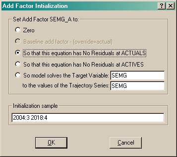
You can edit the add factor in a variety of ways to create the type of shock in line with your intentions. Another useful way to impose shocks is to solve the model so that an endogenous variable follows a predetermined path. Suppose you believe that the imports of goods will develop according to the path of SEMGTARGET. You then create that variable and let BASMOD solve for that:

 

 

which means that the add factor SEMG_A is created such that SEMG=SEMGTARGET.

 

This procedure can also be followed in the event of keeping the policy interest rate constant for, say, 2 years. The following steps are needed.

 

·        Create the target variable SER3MTARGET

·        Let SER3MTARGET=2.01 which is the present policy rate of interest

·        Initialize the add factor as above for the period 2004:3 - 2006:2

·        Run the forecast for the period you wish such as 2004:3 - 2018:4

 

as shown below:

 

 

 

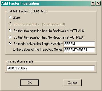
and the model creates SER3M_A such that these shocks (or add factors) to the policy rate of interest generates a constant policy rate for 2004:3 – 2006:2 and an endogenous policy rate without shocks for the period 2006:3 – 2018:4.

 

Several other possibilities are available and the reader is referred to the Eviews manual and help menus.

 

5 How to change the model

 

As briefly mentioned above it is easy to make changes to the model and it can be done in various ways. In the Text view of the Model object equations are written down either directly in text mode or linked from estimated equations:

 

SEC = 0.98 * SEC(-1)

:EKMS

 

where you can get information about the linked equation EKMS either from the Equations view in the Model object:

 

 

or from opening the Equation object for EKMS, in this case the Stats view:

 

 

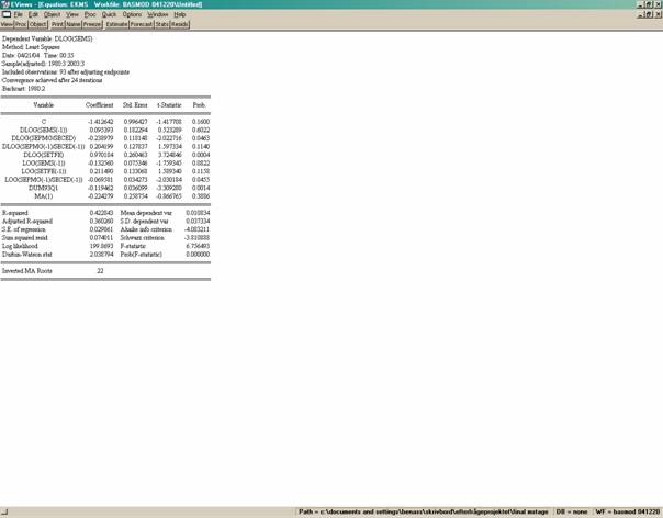
If you for some reason do not want to link the equation as above you can write it in text mode by clicking View/Representations to get

 

 

and copy the last two rows and paste them into the Text view of the Model object to get:

 

SEC = 0.98 * SEC(-1)

DLOG(SEMS) = -1.412642028 + 0.09539261914*DLOG(SEMS(-1)) - 0.2389790551*DLOG(SEPMG/SECED) + 0.2041986262*DLOG(SEPMG(-1)/SECED(-1)) + 0.9701842787*DLOG(SETFE) - 0.1325599308*LOG(SEMS(-1)) + 0.2114900038*LOG(SETFE(-1)) - 0.06958096575*LOG(SEPMG(-1)/SECED(-1)) - 0.119461945*DUM93Q1 + [MA(1)=-0.224278931,BACKCAST=1980:3]

 

These equations you can simply edit in the Text view of the Model object. For an estimated equation it is perhaps preferable to reestimate the equation and link the reestimated equation to the model. A convenient procedure is to make a copy of the original equation and give it a new name – e.g. EKMS2 – and link it to the model:

 

SEC = 0.97 * SEC(-1)

:EKMS2

 

Of course you can add new equations to the model by simply writing them in the above format into the Text view of the Model object. If you believe that the coefficient in the consumption equation which was changed from 0.98 to 0.97 is actually changing over time you can run a time varying parameters state space model – e.g. with the name SSC – and replace the original equation by the following link:

 

:SSC

:EKMS2

 

There are a lot of possibilities to change the model in various ways and the changes are easy to implement in BASMOD/Eviews. Note that if you reestimate a linked object and rerun the model you have to recompile the model by clicking Procs/Links/Update All Links – Recompile model to make the changes take effect.

 

6 Further information

 

Further information about how to run the model can be found in the BASMOD home page and also in the chapter on Models in the Eviews user manual.